Category: Education

  • My Journey Building Elasticsearch for Retail

    My Journey Building Elasticsearch for Retail

    If, like me, you’ve taken the journey that is building an Elasticsearch retail project, you’ve inevitably experienced many challenges. Challenges like, how do I index data, use the query API to build facets, page through the results, sorting, and so on? One aspect of optimization that frequently receives too little attention is the correct configuration of search analyzers. Search analyzers define the architecture for a search query. Admittedly, it isn’t straightforward!

    The Elasticsearch documentation provides good examples for every kind of query. It explains which query is best for a given scenario. For example, “Phrase Match” queries find matches where the search terms are similar. Or “Multi Match” with “most field” type are “useful when querying multiple fields that contain the same text analyzed in different ways”.

    All sounds good to me. But how do I know which one to use, based on the search input?

    Elasticsearch works like cogs within a Rolex

    Where to Begin? Search query examples for Retail.

    Let’s pretend we have a data feed for an electronics store. I will demonstrate a few different kinds of search inputs. Afterward, I will briefly describe how search should work in each case.

    Case #1: Product name.

    For example: “MacBook Air

    Here we want to have a query that matches both terms in the same field, most likely the title field.

    Case #2: A brand name and a product type

    For example: “Samsung Smartphone”

    In this case, we want each term to match a different field: brand and product type. Additionally, you want to find both terms as a pair. Modifying the query in this way prevents other smartphones or Samsung products from appearing in your result.

    Case #3: The specific query that includes attributes or other details

    For example: “notebook 16 GB memory”

    This one is tricky because you want “notebook” to match the product type, or maybe your category is named such. On the other hand, you want “16 GB” to match the memory attribute field as a unit. The number “16” shouldn’t match some model number or other attribute.

    For example: “MacBook Pro 16 inch“ is also in the “notebook” category and has some “GB” of “memory“. To further complicate matters, search texts might not contain the term “memory”, because it’s the attribute name.

    As you might guess, there are many more. And we haven’t even considered word composition, synonyms, or typos yet. So how do we build one query that handles all cases?

    Know where you come from to know where you’re headed

    Preparation

    Before striving for a solution, take two steps back and prepare yourself.

    Analyze your data

    First, take a closer look at the data in question.

    • How do people search on your site?
    • What are the most common query types?
    • Which data fields hold the required content?
    • Which data fields are most relevant?

    Of course, it’s best if you already have a site search running and can, at least, collect query data there. If you don’t have a site search analytics, even access-logs will do the trick. Moreover, be sure to measure which queries work well and which do not provide proper results. More specifically, I recommend taking a closer look at how to implement tracking, the analysis, and evaluation.

    You are welcome to contact us if you need help with this step. We enjoy learning new things ourselves. Adding searchHub to your mix gives you a tool that combines different variations of the same queries (compound & spelling errors, word order variations, etc.). This way, you get a much better view of popular queries.

    Track your progress

    You’ll achieve good results for the respective queries once you begin tuning them. But don’t get complacent about the ones you’ve already solved! More recent optimizations can break the ones you previously solved.

    The solution might simply be to document all those queries. Write down the examples you used, what was wrong with the result before, and how you solved it. Then, perform regression tests on the old cases, following each optimization step.

    Take a look at Quepid if you’re interested in a tool that can help you with that. Quepid helps keep track of optimized queries and checks the quality after each optimization step. This way, you immediately see if you’re about to break something.

    The fabled, elusive silver-bullet.

    The Silver-Bullet Query

    Now, let’s get it done! Let me show you the perfect query that solves all your problems…

    Ok, I admit it, there is none. Why? Because it heavily depends on the data and all the ways people search.

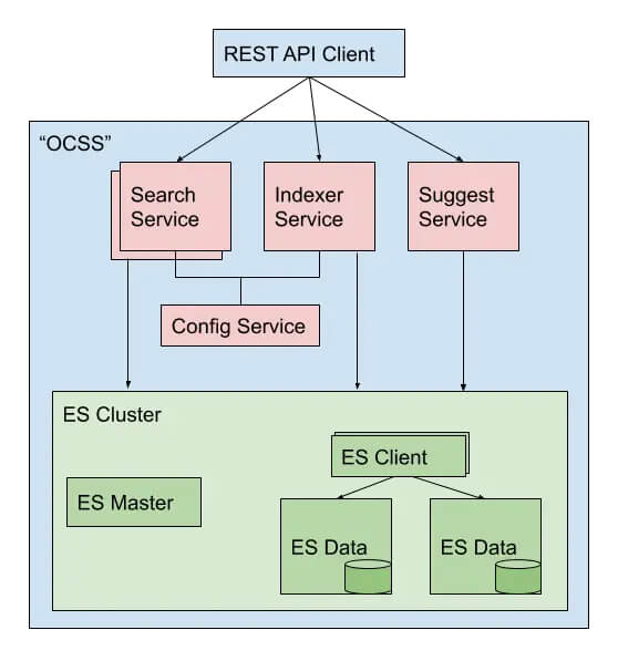
    Instead, I want to share my experience with these types of projects and, in so doing, present our approach to search with Open Commerce Search Stack (OCSS):

    Similarity Setting

    When dealing with structured data, the scoring algorithms of Elasticsearch “TF/IDF” and BM25 will most likely screw things up. These approaches work well for full-text search, like Wikipedia articles or other kinds of content. And, in the unfortunate case where your product data is smashed into one or two fields, you might also find them helpful. However, with OCSS (Open Commerce Search Stack), we took a different approach and set the similarity to “boolean”. This change makes it much easier to comprehend the scores of retrieved results.

    Multiple Analyzers

    Let Elasticsearch analyze your data using different types of analyzers. Do as little normalization as possible and as much as necessary for your base search-fields. Use an analyzer that doesn’t remove information. What I mean with this is no stemming, stop-words, or anything like that. Instead, create sub-fields with different analyzer approaches. These “base fields” should always have a greater weight during search time than their analyzed counterparts.

    The following shows how we configure search data mappings within OCSS:

    				
    					{
      "search_data": {
        "path_match": "*searchData.*",
        "mapping": {
          "norms": false,
          "fielddata": true,
          "type": "text",
          "copy_to": "searchable_numeric_patterns",
          "analyzer": "minimal",
          "fields": {
            "standard": {
              "norms": false,
              "analyzer": "standard",
              "type": "text"
            },
            "shingles": {
              "norms": false,
              "analyzer": "shingles",
              "type": "text"
            },
            "ngram": {
              "norms": false,
              "analyzer": "ngram",
              "type": "text"
            }
          }
        }
      }
    }
    				
    			
    Analyzers used above explained

    Let’s break down the different types of analyzers used above.

    • The base field uses a customized “minimal” analyzer that removes HTML tags, non-word characters, transforms the text to lowercase, and splits it by whitespaces.
    • With the subfield “standard”, we use the “standard analyzer” responsible for stemming, stop words, and the like.
    • With the subfield “shingles”, we deal with unwanted composition within search queries. For example, someone searches for “jackwolfskin”, but it’s actually “jack wolfskin”.
    • With the subfield “ngram,” we split the search data into small chunks. We use that if our best-case query doesn’t find anything – more about that in the next section, “Query Relaxation”.
    • Additionally we copy the content to the “searchable_numeric_patterns” field which uses an analyzer that removes everything but numeric attributes, like “16 inch”.

    The most powerful Elasticsearch Query

    Use the “query string query” to build your final Elasticsearch query. This query type gives you all the features from all other query types. In this way, you can optimize your single query without the need to change to another query type. However, it would be best to strip “syntax tokens”; otherwise, you might get an invalid search query.

    Alternatively, use the “simple query string query,” which can also handle most cases if you’re uncomfortable with the above method.

    My recommendation is to use the “cross_fields” type. It’s not suitable for all kinds of data and queries, but it returns good results in most cases. Place the search text into quotes and use a different quote_analyzer to prevent the search input from being analyzed with the same analyzer. Also, if the quoted-string receives a higher weight, a result with a matching phrase is boosted. This is how the query-string could look: “search input “^2 OR search input.

    And remember, since there is no “one query to rule them all,” use query relaxation.

    How do I use Query Relaxation?

    After optimizing a few dozen queries, you realize you have to make some compromises. It’s almost impossible to find a single query that works for all searches.

    For this reason, most implementations I’ve seen opt for the “OR” operator, thus allowing a single term to match when multiple terms are in the search input. The issue here is that you still end up with results that only partially match. It’s possible to combine the “OR” operator with a “minimum_should_match” definition to boost more matches to the top and control the behavior.

    Nevertheless, this may have some unintended consequences. First, it could pollute your facets with irrelevant attributes. For example, the price slider might show a low price range just because the result contains unrelated cheap products. It may also have the unwanted effect of making ranking the results according to business rules more difficult. Irrelevant matches might rank toward the top simply because of their strong scoring values.

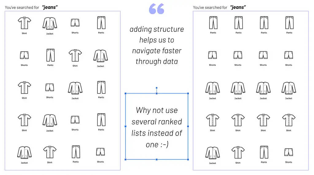
    So instead of the silver-bullet query – build several queries!

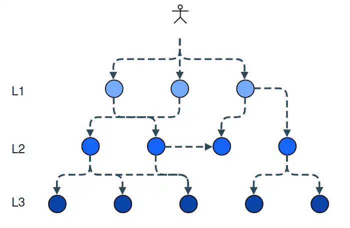
    Relax queries, divide the responsibility, use several

    The first query is the most accurate and works for most queries while avoiding unnecessary matches. Run a second query that is more sloppy and allows partial matches if the initial one leads to zero results. This more flexible approach should work for the majority of the remaining queries. Try using a third query for the rest. Within OCSS, at the final stage, we use the “ngram” query. Doing so allows for partial word matches.

    “But sending three queries to Elasticsearch will need so much time,” you might think. Well, yes, it has some overhead. At the same time, it will only be necessary for about 20% of your searches. Also, zero-matches are relatively fast in their response. They are calculated pretty quickly on 0 results, even if you request aggregations.

    Sometimes, it’s even possible to decide in advance which query works best. In such cases, you can quickly pick the correct query. For example, identifying a numeric search is easy. As a result, it’s simple only to search numeric fields. Also, as there is no need to analyze a second query, it’s easier to handle single-term searches uniquely. Try to improve this process even further by using an external spell-checker like SmartQuery and a query-caching layer.

    Conclusion

    I hope you’re able to learn from my many years of experience; from my mistakes. Frankly, praying your life away (e.g., googling till the wee hours of the morning), hoping, and waiting for a silver-bullet query, is entirely useless and a waste of time. Learning to combine different query analysis types and being able to accept realistic compromises will bring you closer, faster to your desired outcome: search results that convert more visitors, more of the time than what you previously had.

    We’ve shown you several types of analyzers and queries that will bring you a few steps closer to this goal today. Strap in and tune in next week to find out more about OCSS if you are interested in a more automated version of the above.

  • How To DIY Site search analytics – made easy

    How To DIY Site search analytics – made easy

    In my first post, I talked about the importance of site search analytics for e-commerce optimization. In this follow-up, I would like to show one way how to easily build a site search analytics system at scale, without spending much time and effort on answering these ever present questions:

    1. Which database is best for analytics?
    2. How do I operate that database at scale?
    3. What are the operating costs for the database?

    How-To Site-Search Analytics without the Headache

    These questions are important and necessary. Thankfully, in the age of cloud computing, others have already thought about, and found solutions to abstract out the complexity. One of them is Amazon Athena. This will help us build a powerful analysis tool from, in the simplest case, things like CSV files. Amazon Athena, explained in its own words:

    Athena is an interactive query service that makes it easy to analyze data in Amazon S3 using standard SQL. Athena is serverless, so there is no infrastructure to manage, and you pay only for the queries that you run. Amazon Athena

    This introductory sentence from the Amazon website already answers our questions 1 and 2. All that remains is to answer question 3: how much does it cost? This is answered quickly enough:

    • $5.00 per TB of data scanned by Athena
    • Standard AWS S3 rates for storage, requests, and data transfer


    AWS offers a calculator to roughly estimate the cost. Because Amazon Athena uses Presto under the hood, it works with a variety of data formats. This includes CSV, JSON, ORC, Apache Parquet, and Apache Avro. Choosing the right file format can save you up to a third of the cost.

    No data, no DIY analytics

    A site search analytics tool requires a foundation. Either data from an e-commerce system or any site search tracking tool like the searchhub search-collector will suffice. For now, we will focus on how to convert data into the best possible format, and leave the question of “how to extract data from the various systems” for a separate post.

    As the database needn’t scan a complete row but only the columns which are referenced in the SQL query, a columnar data format is preferred to achieve optimal read performance. And to reduce overall size, the file format should also support data compression algorithms. In the case of Athena, this means we can choose between ORC, Apache Parquet, and Apache Avro. The company bryteflow provides a good comparison of these three formats here. These file formats are efficient and intelligent. Nevertheless, they lack the ability to easily inspect the data in a humanly readable way. For this reason, consider adding an intermediate file format to your ETL pipeline. Use this file to store the original data in an easy-to-read format like CSV or JSON. This will make your life easier when debugging any strange-looking query results.

    What are we going to build?

    We’ll now build a minimal Spring Boot web application that is capable of the following:

    1. Creating dummy data in a humanly readable way
    2. Converting that data into Apache Parquet
    3. Uploading the Parquet files to AWS S3
    4. Query the data from AWS Athena using JOOQ for creating type-safe SQL queries using the Athena JDBC driver.

    Creating the application skeleton

    Head over to Spring initializr and generate a new application with the following dependencies:

    • Spring Boot DevTools
    • Lombok
    • Spring Web
    • JOOQ Access Layer
    • Spring Configuration Processor

    Hit the generate button to download the project. Afterward, you need to extract the zip file and import the maven project into your favorite IDE.

    Our minimal database table will have the following columns:

    1. query
    2. searches
    3. clicks
    4. transactions


    We will use the jooq-codegen-maven plugin, to build type-safe queries with JOOQ, which will generate the necessary code for us. The plugin can be configured to generate code based on SQL DDL commands. Create a file called jooq.sql inside src/main/resources/db and add the following content to it:

    				
    					CREATE TABLE analytics (
        query VARCHAR,
        searches INT ,
        clicks INT,
        transactions INT,
        dt VARCHAR
    );


    Next, add the plugin to the existing build/plugins section of our projects pom.xml:

    				
    					<plugin>
        <groupId>org.jooq</groupId>
        <artifactId>jooq-codegen-maven</artifactId>
        <executions>
            <execution>
                <id>generate-jooq-sources</id>
                <phase>generate-sources</phase>
                <goals>
                    <goal>generate</goal>
                </goals>
                <configuration>
                    <generator>
                        <generate>
                            <pojos>true</pojos>
                            <pojosEqualsAndHashCode>true</pojosEqualsAndHashCode>
                            <javaTimeTypes>true</javaTimeTypes>
                        </generate>
                        <database>
                            <name>org.jooq.meta.extensions.ddl.DDLDatabase</name>
                            <inputCatalog></inputCatalog>
                            <inputSchema>PUBLIC</inputSchema>
                            <outputSchemaToDefault>true</outputSchemaToDefault>
                            <outputCatalogToDefault>true</outputCatalogToDefault>
                            <properties>
                                <property>
                                    <key>sort</key>
                                    <value>semantic</value>
                                </property>
                                <property>
                                    <key>scripts</key>
                                    <value>src/main/resources/db/jooq.sql</value>
                                </property>
                            </properties>
                        </database>
                        <target>
                            <clean>true</clean>
                            <packageName>com.example.searchinsightsdemo.db</packageName>
                            <directory>target/generated-sources/jooq</directory>
                        </target>
                    </generator>
                </configuration>
            </execution>
        </executions>
        <dependencies>
            <dependency>
                <groupId>org.jooq</groupId>
                <artifactId>jooq-meta-extensions</artifactId>
                <version>${jooq.version}</version>
            </dependency>
        </dependencies>
    </plugin>


    The IDE may require the maven project to be updated before it can be recompiled. Once done, you should be able to see the generated code under target/generated-sources/jooq.

    Before creating SQL queries with JOOQ, we first need to create a DSL-context using an SQL connection to AWS Athena. This assumes we have a corresponding Athena JDBC driver on our classpath. Unfortunately, maven central provides only an older version (2.0.2) of the driver, which isn’t an issue for our demo. For production, however, you should use the most recent version from the AWS website. Once finished, publish it to your maven repository. Or add it as an external library to your project, if you don’t have a repository. Now, we need to add the following dependency to our pom.xml:

    				
    					<dependency>
        <groupId>com.syncron.amazonaws</groupId>
        <artifactId>simba-athena-jdbc-driver</artifactId>
        <version>2.0.2</version>
    </dependency>


    Under src/main/resources rename the file application.properties to application.yml and paste the following content into it:

    				
    					spring:
      datasource:
        url: jdbc:awsathena://<REGION>.amazonaws.com:443;S3OutputLocation=s3://athena-demo-qr;Schema=demo
        username: ${ATHENA_USER}
        password: ${ATHENA_SECRET}
        driver-class-name: com.simba.athena.jdbc.Driver


    This will auto-configure a JDC connection to Athena and Spring will provide us a DSLContext bean which we can auto-wire into our service class. Please note that I assume you have an AWS IAM user that has access to S3 and Athena. Do not store sensitive credentials in the configuration file, rather pass them as environment variables to your application. You can easily do this, if working with Spring Toll Suite. Simply select the demo application from the Boot Dashboard; then the pen icon to open the launch configuration; navigate to the Environment tab and add the following entries:

    Please note the datasource URL property, where you need to add proper values for the following placeholders directly in your properties.yml:

    1. REGION: The region you created your Athena database in. We will cover this step shortly.
    2. S3OutputLocation: The bucket where Athena will store query results.
    3. Schema: The name of the Athena database we are going to create shortly.


    We are about to load our Spring Boot application. Our Athena database is still missing, however. And the application won’t start without it.

    Creating the Athena database

    Login to the AWS console and navigate to the S3 service. Hit the Create bucket button and choose a name for it. You won’t be able to use the same bucket as in this tutorial because S3 bucket names must be unique. However, the concept should be clear. For this tutorial, we will use the name, search-insights-demo and skip any further configuration. This is the location to where we will, later, upload our analytics files. Press Create bucket, and navigate over to the Athena service.

    Paste the following SQL command into the New query 1 tab:

    CREATE DATABASE IF NOT EXISTS demo;

    Hit Run query. The result should look similar to this:

    Now, that we have successfully created a database open the Database drop-down on the left-hand side and select it. Next we create a table by running the following query:

    				
    					CREATE EXTERNAL TABLE IF NOT EXISTS analytics (
        query STRING,
        searches INT ,
        clicks INT,
        transactions INT
    )
    PARTITIONED BY (dt string)
    STORED AS PARQUET
    LOCATION 's3://search-insights-demo/'


    The result should look similar to this:

    Please note some important details here:

    1. We partition our table by a string called dt. By partitioning, we can restrict the amount of data scanned by each query. This improves performance and reduces cost. Analytics data can be partitioned perfectly into daily slices.
    2. We state that our stored files are in Apache Parquet format.
    3. We point the table to the previously created S3 bucket. Please adjust the name to the one you have chosen. Important: the location must end with a slash otherwise you will face an IllegalArgumentException.

    Adding the first query to our application

    Now, that everything is setup we can add a REST controller to our application that counts all records in our table. Naturally, the result we expect is 0 as we have yet to upload any data. But this is enough to prove that everything is working.

    Now, return to the IDE and, in the package com.example.searchinsightsdemo.service, create a new class called AthenaQueryService and paste the following code into it:

    				
    					package com.example.searchinsightsdemo.service;
    import static com.example.searchinsightsdemo.db.tables.Analytics.ANALYTICS;
    import org.jooq.DSLContext;
    import org.springframework.beans.factory.annotation.Autowired;
    import org.springframework.stereotype.Service;
    @Service
    public class AthenaQueryService {
        @Autowired
        private DSLContext context;
        public int getCount() {
            return context.fetchCount(ANALYTICS);
        }
    }


    Note that we auto-wire the DSLContext which Spring Boot has already auto-configured based on our settings in the properties.yml. The service contains one single method that uses the context to execute a fetch count query on the ANALYTICS table, which the JOOQ code generator has already created (see the static import).

    A Spring service is nothing without a controller exposing it to the outside world, so let’s create a new class, in the package com.example.searchinsightsdemo.rest, called AthenaQueryController. Go there now and add the following:

    				
    					@RestController
    @RequestMapping("/insights")
    public class AthenaQueryController {
        @Autowired
        private AthenaQueryService queryService;
        @GetMapping("/count")
        public ResponseEntity<Integer> getCount() {
            return ResponseEntity.ok(queryService.getCount());
        }
    }


    Nothing special here. Just some Spring magic that exposes the REST endpoint /insights/count. This in turn calls our service method and returns the results as a ResponseEntity.

    We need to add one more configuration block to the properties.yml, before launching the application for the first time:

    				
    					logging:
      level:
        org.jooq: DEBUG


    This will enable debug logging for JOOQ which enables viewing the SQL queries it generates as plain text in our IDE’s console.

    That was quite a piece of work. Fingers crossed that the application boots. Give it a try by selecting it in the Boot Dashboard and pressing the run button. If everything works as expected you should be able to curl the REST endpoint via:

    curl -s localhost:8080/insights/count

    The response should match the expected value of 0, and you should be able to see the following log message in your console:

    				
    					Executing query          : select count(*) from "ANALYTICS"
    Fetched result           : +-----+
                             : |count|
                             : +-----+
                             : |    0|
                             : +-----+                                                                  
    Fetched row(s)           : 1   


    Summary

    In this first part of our series, we introduced AWS Athena as a cost-effective way of creating an analytics application. We illustrated how to build this yourself by using a Spring Boot web application and JOOQ for type-safe SQL queries. The application hasn’t any analytics capabilities so far. This will be added in part two where we create fake data for the database. To achieve this, we will first show how to create Apache Parquet files; partition them by date, and upload them via AWS S3 Java SDK. Once uploaded, we will look at how to inform Athena about new data.

    Stay tuned and come back soon!

    The source code for part one can be found on GitHub.

  • Part 2: Search Quality for Discovery & Inspiration

    Part 2: Search Quality for Discovery & Inspiration

    Series: Three Pillars of Search Quality in eCommerce

    In the first part of our series, we learned about Search Quality dimensions. We then introduced the Findability metric, and explained the relationship of this metric on search quality. This metric is helpful when considering how well your search engine handles the information retrieval step. Unfortunately, it completely disregards the emotionally important discovery phase. Essential for both eCommerce, as well as retail in general. In order to better grasp this relationship we need to understand how search quality influences discovery and inspiration.

    What is the Secret behind the Most Successful high-growth Ecommerce Shops?

    If we analyze the success of high-growth shops, three unique areas set them apart from their average counterparts.

    Photo by Sigmund on Unsplash – if retail could grow like plants

    What Separates High-Growth Retail Apart from the Rest?

    1. Narrative: The store becomes the story

    Your visitors are not inspired by the same presentation of trending products every time they land on your site. What’s the use of shopping if a customer already knows what’s going to be offered (merchandised) to them?

    Customers are intrigued by visual merchandising which is, in essence, brand storytelling. Done correctly, this will transform a shop into an exciting destination that both inspires, as well as entices shoppers. An effective in-store narrative emotionally sparks customers’ imagination, while leveraging store ambience to transmit the personality of the brand. Perhaps using a “hero” to focus attention on a high-impact collection of bold new items. Or an elaborate holiday display that nudges shoppers toward a purchase.

    Shopping is most fun, and rewarding, when it involves a sense of discovery or journey. Shoppers are more likely to return when they see new merchandise related to their tastes, and local or global trends.

    2. Visibility: What’s seen is sold (from pure retrieval to inspiration)

    Whether in-store or online, visibility encourages retailers to feature items that align with a unique brand narrative. All the while helping shoppers easily and quickly find the items they’re after. The principle of visibility prioritizes which products retailers push the most. Products with a high margin or those exclusive enough to drive loyalty, whether by word of mouth, or social sharing.

    Online, the e-commerce information architecture, and sitemap flow, help retailers prominently showcase products most likely to sell. This prevents items from being buried deep in the e-commerce site. Merchandisers use data analytics to know which products are most popular and trending. This influences which items are most prominently displayed. These will be the color palettes, fabrics, and cuts that will wow shoppers all the way to the checkout page.

    So why treat search simply as a functional information retrieval tool? Try rethinking it from the perspective of how a shopper might look for something in a brick and mortar scenario.

    3. Balance: Bringing buyer’s and seller’s interests together in harmony

    In stores and online, successful visual merchandising addresses consumers’ felt needs around things like quality, variety, and sensory appeal. However, deeper emotional aspects like trust are strongly encouraged through online product reviews. These inspire their wants: to feel attractive; to be confident, and hopeful. We can agree that merchandisers’ foremost task, is to attend to merchandise and the associated cues to communicate it properly. It’s necessary to showcase sufficient product variety, while at the same time remaining consistent with the core brand theme. This balancing act requires they strike a happy medium between neither overwhelming nor disengaging their audience.

    An example for the sake of clarity:

    Imagine you are a leading apparel company with a decently sized product catalog. Everyday, a few hundred customers come to your site and search for “jeans”. Your company offers over 140 different types of jeans, about 40 different jeans jackets and roughly 80 jeans shirts.

    Now the big question is: which products deserve the most prominent placement in the search result?

    Indeed this is a very common challenge for our customers. And yet all of them struggle addressing it. But why is it so challenging? Mainly because we are facing a multi-dimensional and multi-objective optimisation problem.

    1. When we receive a query like “jeans”, it is not 100% clear what the user is looking for. Trousers, jackets, shirts, we just don’t know. As a result, we have to make some assumptions. We present different paths for him to discover the desired information, or receive the inspiration she needs. In other words, for the most probable product types “k”, and the given query, we need to identify related products.
    2. Next we find the most probable set of product-types. Then, we need to determine which products are displayed at the top for each corresponding set of products. Which pairs of jeans, jeans jackets and jeans shirts? Or again in a more formal way: for each product type “k” find the top-”n” products related to this product-type and the given query.

    Or in simple words: diversify the result set into multiple result sets. Then, learn to rank them independently.

    Now, you may think this is exactly what a search & discovery platform was built for. But unfortunately, 99% of these platforms are designed to work as single-dimension-rank applications. They retrieve documents for a given query, assign weights to the retrieved documents, and finally rank these documents by weight. This dramatically limits your ability to rank the retrieved documents by your own set of, potentially, completely different dimensions. This is the reason most search results for generic terms tend to look messy. Let’s visualize this scenario to clarify what I mean by “messy”.

    You will agree, the image on the left-hand side, is pretty difficult for a user to process and understand. Even if the ranking is mathematically correct. The reason for this is simple: the underlying natural grouping of product types is lost to the user.

    Diversification of a search for “jeans”

    Now, let’s take a look at a different approach. On the right-hand side, you will notice, we diversify the search result while maintaining the natural product type grouping. Doesn’t this look more intuitive and visually appealing? I will assume you agree. After all, this is the most prominent type of product presentation retail has used over the last 100 years.

    Grouping products based on visual similarity

    You may argue that the customer could easily narrow the offering with facets/filters. Data reveals, however, that this is not always the case – even less so on mobile devices. The big conundrum is that you’ve no clue what the customer wants. To be inspired, to be guided in his buying process or just to quickly transact. Additionally, you never know for sure what type of customer you are dealing with. Even with the new, hot, latest and greatest, stuff called “personalization” – that unfortunately fails frequently. Using visual merchandising puts us into conversation with the customer. We ask her to confirm her interests by choosing a “product type”. Yet another reason why diversification is important.

    Still not convinced, this is what separates high-growth retail from the rest?

    Here is another brilliant example of how you could use the natural grouping by product type to diversify your result. Let’s take a look at a seasonal topic in this case. Another very challenging task. So we give customers the perfect starting point to explore your assortment.

    Row-based diversification – explore product catalog

    If you have ever tried creating such a page, with a single search request, you know this is almost an impossible task. Not to mention trying to maintain the correct facet counts, product stock values, etc.

    However, the approach I am presenting offers so much more. This type of result grouping also solves another well-known problem. The multi-objective optimization ranking problem. Making this approach truly game-changing.

    What’s a Multi-Objective Optimization Problem?

    Never heard of it? Pretend for a moment you are the customer. This time you’re browsing a site searching for “jeans”. The type you have in mind is something close to trousers. Unaware of all the different types of jeans the shop has to offer, you have to go rogue. This means navigating your way through new territory to the product you are most interested in. Using filters and various search terms for things like color, shape, price, size, fabric, and the like. Keep in mind that you can’t be interested in what you can’t see. At the same time, you may be keeping an eye on the best value for your money.

    We now turn the table and pick up from the seller’s perspective. As a seller, you want to present products ranked based on stock, margin, and popularity. If you run a well-oiled machine, you may even throw in some fancy Customer Lifetime Value models.

    So, our job is to strike the right balance between the seller’s goals and the customer’s desire. The methodology that attempts to strike such a balance is called the multi-objective optimization problem in ranking.

    Let’s use a visualization to illustrate a straightforward solution to the problem, by a diversified result-set grouping.

    Row-based ranking diversification

    Interested in how this approach could be integrated into your Search & Discovery Platform? Reach out to us @searchHub. Our Beta-Testphase for the Visual-Merchandising open-source module, for our OCSS (Open Commerce Search Stack), begins soon. We hope to use this to soon help deliver more engaging and joyful digital experiences.

    High-Street Visual Merchandising Wisdom Come Home to Roost

    This is all nothing new, rather it’s simply never found its way into digital retailing. For decades, finding the right diversified set of products to attract window shoppers, paired with the right location, was the undisputed most important skill in classical high street retail. Later, this type of shopping engagement was termed “Visual Merchandising”. The process of closing the gap between what the seller wants to sell and what the customer will buy. And of course, how best to manufacture that desire.

    Visual merchandising is one of the most sustainable, as well as differentiating, core assets of the retail industry. Nevertheless, it remains totally underrated.

    Still don’t believe in the value of Visual Merchandising? Give me a couple of sentences and one more Chart to validate my assumptions.

    Before I present the chart to make you believe, we need to align on some terminology.

    Product Exposure Rate (PER): The goal of the product exposure rate is to measure if certain products are under- or over-exposed in our store. The product exposure rate is the “sum of all product views for a given product” divided by “the sum of all product views from all products”.

    Product Net Profit Margin (PNPM): With this metric, we try to find the products with the highest Net Profit Margin. Please be aware: it’s sensible to include all product related costs in your calculation. Customer Acquisition Costs, cost of Product returns, etc. The Product Net Profit Margin is the “Product Revenue” minus “All Product Costs” divided by the “Product Revenue”.

    Now that we have established some common ground, let’s continue calculating these metrics for all active products you sell. We will then visualize them in a graph.

    Product Exposure Rate vs. Product Net Profit Margin

    The data above represents a random sample of 10,000 products from our customers. It may look a bit different for your product data, but the overall tendency should be similar. Please reach out to me if this is not the case! According to the graph it seems that the products with high PER (Product Exposure Rate) tend to have a significantly lower PNPM (Product Net Profit Margin).

    We were able to spot the following two reasons as the most important for this behaviour:

    Two Reasons for Significantly Low Product Net Profit Margin

    1. Higher Customer Acquisition Costs for trending products mainly because of competition. Because of this you may even spot several products with a negative PNPM.
    2. Another reason is the natural tendency for low priced products to dominate the trending items. This type of over-exposure encourages high-value visitors, to purchase cheaper trending products with a lower PNPM. Customers to whom you would expect to sell higher margin products under normal circumstances.

    I simply can’t over-emphasize how crucial digital merchandising is for a successful and sustainable eCommerce business. This is the secret weapon for engaging your shoppers and guiding them towards making a purchase. To take full advantage of the breadth of your product catalog, you must diversify and segment. Done intelligently, shoppers are more likely to buy from you. Not only that, they’ll also enjoy engaging with, and handing over their hard-earned money to your digital store. For retailers, this means a significant increase in conversions, higher AOV, higher margins, and more loyal customers.

    Conclusion

    Initially, I was going to close this post right after describing how this problem can be solved, conceptually. However, I would have missed an essential, if not the most important part of the story.

    Yes, we all know that we live in a data-driven world. Believe me, we get it. At searchHub, we process billions of data points every day to help our customers understand their users at scale. But in the end, data alone won’t make you successful. Unless, of course, you are in the fortunate position of having a data monopoly.

    To be more concrete: data will/can help you spot or detect patterns and/or anomalies. It will also help you scale your operations more efficiently. But there are many areas where data can’t help. Especially when faced with sparse and biased data. In retail this is the kind of situation we are essentially dealing with 80% of the time. All digital Retailers, of which I am aware, with a product catalog greater than 10,000 SKUs, face the product exposure bias. This means, only 50-65% of the 10.000 SKUs will ever be seen (exposed) by their users. The rest remain hidden somewhere in the endless digital aisle. Not only does this cost money, it also means a lot of missed potential revenue. Simply put: you can’t judge the value of a product that has never been seen. Perhaps it could have been the Top-Seller you were always looking for were it only given the chance to shine?

    Keep in mind that retailers offer a service to their customers. Only two things make customers loyal to a service.

    What makes loyal customers?

    • deliver a superior experience
    • be the only one to offer a unique type of service

    Being the one that “also” offers the same type of service won’t help to differentiate.

    I’m one hundred percent sure that today’s successful retail & commerce players are the ones that:

    1. Grasp the importance of connecting brand and commerce
    2. Comprehend how shoppers behave
    3. Learn their data inside and out
    4. Develop an eye for the visual
    5. Connect visual experiences to business goals
    6. Predict what shoppers will search for
    7. Understand the customer journey and how to optimize for it
    8. Think differently when it comes to personalizing for customers
    9. Realize it’s about the consumer, not the device or channel

    I can imagine many eCommerce Managers might feel overwhelmed by the thought of delivering an eCommerce experience that sets their store apart. I admit, it’s a challenge connecting all those insights and capabilities practically. And while we’re not going to minimize the effort involved, we have identified an area that will elevate your digital merchandising to new levels and truly differentiate you from the competition.

  • The Art of Abstraction – Revisiting Webshop Architecture

    The Art of Abstraction – Revisiting Webshop Architecture

    Why Abstraction is Necessary for Modern Web Architecture

    Why abstraction, and why should I reconsider my web-shop architecture? In the next few minutes, I will attempt to lay clear the increase in architectural flexibility, and the associated profit gains. This is especially true when abstraction is considered foundational rather than cosmetic, operational, or even departmental.

    TL;DR

    Use Abstraction! It will save you money and increase flexibility!

    OK, that was more of a compression than an abstraction 😉

    The long story – abstraction a forgotten art

    The human brain is bursting with wonder all its own. Just think of the capabilities each of us has balanced between our shoulders.

    One such capability is the core concept of using abstraction to grasp the complex world around us and store it in a condensed way.

    This, in turn, makes it possible for us humans to talk about objects, structures, and concepts which would be impossible if we had to cope with all the details all the time.

    What is Abstraction?

    Abstraction is also one of the main principles of programming, making software solutions more flexible, maintainable and extensible.

    We programmers are notoriously lazy. As such, not reinventing the wheel is one of the major axioms by which each and every one of us guides our lives by.

    Besides saving time, abstraction also reduces the chance of bugs. As a result, should you find any crawling around inside your code, you simply need to squash them in one location, not multiple times over and over again, provided you’ve got your program structure right.

    Using abstract definitions to derive concrete implementations helps accomplish precisely this.

    Where have you forgotten to implement abstraction?

    Nevertheless, there is one location where you might not be adhering to this general concept of abstraction: the central interface between your shop and your underlying search engine. Here you may have opted for quick integration, over decoupled code. As a result, you’ve most likely directly linked these two systems, as in the image below. Search Engines sit atop Webshop architecture, which is most often abstracted.

    Perhaps you were lucky enough, when you opened the API documentation of your company’s proprietary site-search engine, to discover well-developed APIs making the integration easy like Sunday morning.

    However, I want to challenge you to consider what there is to gain, by adding another layer of abstraction between shop and search engine.

    Who needs more abstraction? Don’t make my life more complicated!

    At first, you might think, why should I add yet another program or service to my ecosystem. Isn’t that just one more thing I need to take care of?

    This depends heavily on what your overall system looks like. For a small pure player online shop, you may be right.

    However, the bigger you grow, the more consumers of search results you have. Naturally, this increases the number of search results and related variations across the board. It follows, that the need, within your company, to enhance or manipulate the results will grow congruently. A situation like this markedly increases the rate at which your business stands to profit from abstracted access to the search engine.

    One of the main advantages of structuring your system in this way is the greater autonomy you achieve from the site search engine.

    Why do I want search engine autonomy?

    At this point, it’s necessary to mention that site-search engines, largely, provide the same functionality. Each in its own unique way, of course. So, where’s the problem?

    Site-Search APIs are unlikely to be the same among different engines. Whether you compare open source solutions like Solr to Elasticsearch, or commercial solutions like Algolia, FACT-Finder, Fredhopper to whatever else. Switching between or migrating systems will be a bear.

    But why is that? All differences aside, the site-search engine use case is the same across the board. Core functionalities must be consistent:

    • searching
    • category navigation
    • filtering
    • faceting
    • sorting
    • suggesting

    Site-Search abstraction puts the focus on core functionalities – not APIs

    The flexibility you gain through an abstraction-based solution cannot be underplayed.

    Once you have created a layer to abstract out these functionalities and made them generally usable for every consumer of search within your company, it is simple to integrate any other solution and switch over just like that.

    And, since there is no need to deeply integrate the different adapters into your shop’s software, you can more easily enable simple A/B tests.

    Furthermore, if another department also integrates search functionalities, it could be easier for them to use your well-designed abstracted API without re-inventing the wheel locally. Details like, “how does Solr create facets”, or “how do I boost the matching terms in a certain field”, do not need to be rehashed by each department.

    Solve this once in your abstraction layer, and everyone profits.

    A real-world example worth having a look at is our Open Commerce Search Stack (OCSS). You can find an overview of the architecture in a previous blog post [https://blog.searchhub.io/introducing-open-commerce-search-stack-ocss]. The OCSS abstracts the underlying Elasticsearch component and makes it easier to use and integrate. And, because this adapter is Open Source, it can also be used for other search solutions.

    By the way, this method also gives the ability to add functionalities on top. An advantage which cannot be overstated. Let’s have a look at a couple.

    Examples of increased webshop flexibility with increased abstraction:

    • You want to add real-time prices from another data source to the results found? Just add this as a post-processing step after the search engine retrieved the list of products.
    • You want to map visitor queries to their best performing equivalent with our SmartQuery solution? Easy! Just plug in our JAR file, add a few lines of code, and BAAAM, you’re done.


    This also enables the use of our redirect module, getting your customers to the right target page with campaigns, content, or the category they are looking for.

    Oh, and if you simply want to version update your engine, any related API changes can be “hidden” from the consuming services, making it easy to stay up to date. Or at least making new features an optional enhancement that every department can start using whenever they have the time to integrate the necessary changes and switch to the new version of your centrally abstracted API.

    Conclusion

    Depending on the complexity of your webshop’s ecosystem and the variety of services you already use or plan to integrate, abstracting the architecture of your internal site-search solution and related connections can make a noticeable difference.

    In the long run, it can save you a lot of time, and headaches. And in the end increase profits without having to reinvent the wheel.

  • Monitor Elasticsearch in Kubernetes Using Prometheus

    Monitor Elasticsearch in Kubernetes Using Prometheus

    In this article, I will show how to monitor Elasticsearch running inside Kubernetes using the Prometheus-operator, and later Grafana for visualization. Our sample will be based on the cluster described in my last article.

    There are plenty of businesses that have to run and operate Elasticsearch on their own. This can be solved pretty well, because of the wide range of deployment types and the large community (an overview here). However, if you’re serious about running Elasticsearch, perhaps as a critical part of your application, you MUST monitor. In this article, I will show how to monitor Elasticsearch running inside Kubernetes using Prometheus as monitoring software. We will use the Prometheus-operator for Kubernetes, but it will work with a plain Prometheus in the same way.

    Overview of Elasticsearch Monitoring using Prometheus

    If we talk about monitoring Elasticsearch, we have to keep in mind, that there are multiple layers to monitor:

    It is worth noting that every one of these methods uses the Elasticsearch internal stats gathering logic to collect data about the underlying JVM and Elasticsearch itself.

    The Motivation Behind Monitoring Elasticsearch Independently

    Elasticsearch already contains monitoring functionality, so why try to monitor Elasticsearch with an external monitoring system? Some reasons to consider:

    • If Elasticsearch is broken, the internal monitoring is broken
    • You already have a functioning monitoring system with processes for alerting, user management, etc.

    In our case, this second point was the impetus for using Prometheus to monitor Elasticsearch.

    Let’s Get Started – Install the Plugin

    To monitor Elasticsearch with Prometheus, we have to export the monitoring data in the Prometheus exposition format. To this end, we have to install a plugin in our Elasticsearch cluster which exposes the information in the right format under /_prometheus/metrics. If we are using the Elasticsearch operator, we can install the plugin in the same way as the S3 plugin, from the last post, using the init container:

    				
    					version: 7.7.0
     ...
     nodeSets:
     - name: master-zone-a
       ...
       podTemplate:
         spec:
           initContainers:
           - name: sysctl
             securityContext:
               privileged: true
             command: ['sh', '-c', 'sysctl -w vm.max_map_count=262144']
           - name: install-plugins
             command:
             - sh
             - -c
             - |
               bin/elasticsearch-plugin install -b repository-s3 https://github.com/vvanholl/elasticsearch-prometheus-exporter/releases/download/7.7.0.0/prometheus-exporter-7.7.0.0.zip
       ...


    If you are not using the Elasticsearch-operator, you have to follow the Elasticsearch plugin installation instructions.

    Please note: there is more than one plugin on the market for exposing elasticsearch monitoring data in the Prometheus format, but the Elasticsearch-prometheus-exporter we are using is one of the larger projects which is active and has a big community.

    If you are using elasticsearch > 7.17.7 (including 8.x), take a look at the following plugin instead: https://github.com/mindw/elasticsearch-prometheus-exporter/

    After installing the plugin, we should now be able to fetch monitoring data from the /_prometheus/metrics endpoint. To test the plugin, we can use Kibana to perform a request against the endpoint. See the picture below:

    How To Configure Prometheus

    At this point, it’s time to connect Elasticsearch to Prometheus. Now, we can create a ServiceMonitor because we are using the Prometheus-operator for monitoring internal Kubernetes applications. See an example below, which can be used to monitor the Elasticsearch cluster we created in my last post:

    				
    					apiVersion: monitoring.coreos.com/v1
    kind: ServiceMonitor
    metadata:
     labels:
       app: prometheus
       prometheus: kube-prometheus
       chart: prometheus-operator-8.13.8
       release: prometheus-operator
     name: blogpost-es
     namespace: monitoring
    spec:
     endpoints:
       - interval: 30s
         path: "/_prometheus/metrics"
         port: https
         scheme: https
         tlsConfig:
           insecureSkipVerify: true
         basicAuth:
           password:
             name: basic-auth-es
             key: password
           username:
             name: basic-auth-es
             key: user
     namespaceSelector:
       matchNames:
       - blog
     selector:
       matchLabels:
         common.k8s.elastic.co/type: elasticsearch
         elasticsearch.k8s.elastic.co/cluster-name: blogpost


    For those unfamiliar with the Prometheus-operator or are using plain Prometheus to monitor Elasticsearch. The ServiceMonitor will create a Prometheus job like the one below:

    				
    					- job_name: monitoring/blogpost-es/0
      honor_timestamps: true
      scrape_interval: 30s
      scrape_timeout: 10s
      metrics_path: /_prometheus/metrics
      scheme: https
      kubernetes_sd_configs:
      - role: endpoints
        namespaces:
          names:
          - blog
      basic_auth:
        username: elastic
        password: io3Ahnae2ieW8Ei3aeZahshi
      tls_config:
        insecure_skip_verify: true
      relabel_configs:
      - source_labels: [__meta_kubernetes_service_label_common_k8s_elastic_co_type]
        separator: ;
        regex: elasticsearch
        replacement: $1
        action: keep
      - source_labels: [__meta_kubernetes_service_label_elasticsearch_k8s_elastic_co_cluster_name]
        separator: ;
        regex: ui
        replacement: $1
        action: keep
      - source_labels: [__meta_kubernetes_endpoint_port_name]
        separator: ;
        regex: https
        replacement: $1
        action: keep
      - source_labels: [__meta_kubernetes_endpoint_address_target_kind, __meta_kubernetes_endpoint_address_target_name]
        separator: ;
        regex: Node;(.*)
        target_label: node
        replacement: ${1}
        action: replace
      - source_labels: [__meta_kubernetes_endpoint_address_target_kind, __meta_kubernetes_endpoint_address_target_name]
        separator: ;
        regex: Pod;(.*)
        target_label: pod
        replacement: ${1}
        action: replace
      - source_labels: [__meta_kubernetes_namespace]
        separator: ;
        regex: (.*)
        target_label: namespace
        replacement: $1
        action: replace
      - source_labels: [__meta_kubernetes_service_name]
        separator: ;
        regex: (.*)
        target_label: service
        replacement: $1
        action: replace
      - source_labels: [__meta_kubernetes_pod_name]
        separator: ;
        regex: (.*)
        target_label: pod
        replacement: $1
        action: replace
      - source_labels: [__meta_kubernetes_service_name]
        separator: ;
        regex: (.*)
        target_label: job
        replacement: ${1}
        action: replace
      - separator: ;
        regex: (.*)
        target_label: endpoint
        replacement: https
        action: replace


    Warning!: in our example, the scrap interval is 30 seconds. It may be necessary to adjust the interval for your production cluster. Proceed with caution! Gathering information for every scrape creates a heavy load on your Elasticsearch cluster, especially on the master nodes. A short scrape interval can easily kill your cluster.

    If your configuration of Prometheus was successful, you will now see the cluster under the “Targets” section of Prometheus under “All”. See the picture below:

    Import Grafana-Dashboard

    Theoretically, we are now finished. However, because most people out there use Prometheus with Grafana, I want to show how to import the dashboard especially made for this plugin. You can find it here on grafana.com. The screenshots below explain how to import the Dashboard:


    Following the dashboard import, you should see the elasticsearch monitoring graphs as in the following screenshot:

    Wrapping Up

    In this article, we briefly covered the possible monitoring options. I showed why it makes sense to monitor elasticsearch using an external monitoring system and some reasons for doing so. Finally, I showed how to monitor Elasticsearch with Prometheus and Grafana for visualization.

  • Introducing Open Commerce Search Stack – OCSS

    Introducing Open Commerce Search Stack – OCSS

    Why Open-Source (also) Matters in eCommerce

    There are plenty of articles already out there that dig into this question and list the different pros and cons. But as in most cases, the honest answer is “it depends”. So, I want to keep it short and pick – from my perspective – the biggest advantage and the main disadvantage of using open source in the context of eCommerce – or more specifically when it comes to a search solution. Along the way, I’m introducing the Open Commerce Search Stack (OCSS) and show, how it leverages that advantage and reduces the disadvantage. Let’s dig in!

    Pro: Don’t Reinvent the Wheel

    Search is quite a complex topic. Even for bigger players, it requires a lot of time to build something new. There are already outstanding open-source solutions available. No matter if you’re eager to use some fancy AI or just a standard search solution. However, your solution won’t make a difference as long as it hasn’t solved the basic issues.

    In the case of e-commerce search, these are things like data indexation, synonym handling, and faceting. Not to forget operational topics like high availability and scalability. Even companies with a strong focus on search have failed in this area. So why bother with that stuff, when you can get it for free?

    Solutions like Solr and Elasticsearch offer a good basis to get started with the essentials. In this way, you can implement the nice ideas and special features that differentiate your solution. In my opinion this is what matters in the end, and where SaaS solutions come to their limit: you can only ever get as good as the SaaS service you’re using.

    Con: Steep learning curve

    In contrast to a paid SaaS solution, an open-source solution requires you to take care of everything on your own. Without the necessary knowledge and experience, it will be hard to come to a comparable or competitive result. In most cases, it takes time to fully understand the technology and to get it up and running. And even after you have understood what you’re doing, you need take a long hard path to create an outstanding solution. Not to mention the operational side of things, which needs to be taken care of – like forever.

    Where we see demand for a search solution

    So, why are we building the next search solution? A few years ago, we started a proof of concept to see if and how we can build a product search solution with Elasticsearch. We found a very nice guideline and implemented most of it. But even with that guideline and some years of experience, it took us quite a few months to get to a feasible solution.

    The most significant difference to most SaaS solutions is the complex API of Elasticsearch. To get at least some relevant results, you have to build the correct elasticsearch-queries respective of the search query. The same applies to getting the correct facets and to implement filtering correctly and so on. It’s mostly the same case for Solr. As a result, someone unfamiliar with these topics, is going to need more time to get it right. In comparison, proprietary solutions come with impressive REST APIs that only require basic search and filter information.

    We are introducing Open Commerce Search Stack into this gap: a slim layer between your platform and existing open-source solutions. It comes with a simple API for indexation and searching. This way it hides all the complexity of search. Instead of reinventing the wheel, we care about building a nice tire – so to speak – for existing wheel rims out there. At the same time, we lower the learning curve. The result is a solution to get you up and running more quickly without having to mess with all the tiny details. Of course, it also comes with all the other advantages of open source, like flexibility and extendibility, so you always have the option to dive deeper.

    Our Goals for Open Commerce Search Stack

    To sum it up, these are the main goals we focused on when building the OCSS:

    • Extend what’s there: To this end, we take Elasticsearch off the shelf and use best practices to focus only on filling the gaps.
    • Lower the learning curve: With a simple API on top of our solution we hide the complexity of building the correct queries to achieve relevant results. We also prepared a default configuration, that should fit 80% of all use-cases.
    • Keep it flexible: All the crucial parts are configurable. But with batteries included: the stack already comes with a proved and tested default configuration.
    • Keep it extendible: We plan to implement some minimal plugin mechanics to run custom code for indexation, query creation, and faceting.
    • Open for change: With separated components and the API-first approach, we don’t bind to the usage of Elasticsearch. For example we used pure Lucene to build the Auto-Suggest functionality. So it is easy to adopt other search solutions (even proprietary ones) using that API.

    Open Commerce Search Stack – Architecture Overview

    We’re just at the start, so there are only basic components in place. But more are on the horizon. Already, it’s possible to fulfill the major requirements for a search solution.

    • Indexer Service: Takes care of transforming standard key-value data into the correct structure, perfectly prepared for the search service. All controlled by configuration – even some data wrangling logic.
    • Search Service: Hidden behind the simple Search API (you can start with “q=your+term”) a quite complex logic cares about the results. It analyzes the passed search terms and, depending on their characteristic, it uses different techniques to search the indexed data. It also contains “fallback queries” that try some query relaxation in case the first try didn’t succeed.
    • Auto-Suggest: With a data-pull approach, it’s independent of Elasticsearch and still scalable. We use the same service to build our SmartSuggest module, but with cleansed and enriched searchHub data.
    • Configuration Service: Since the Indexer and Search Service are built with Spring Boot, we use Spring Cloud Config to distribute the configuration to these services. However, we’re already planning to build a solution that also allows changing the configuration – of course with a nice REST API. 🙂


    You are welcome to take a look at the current state. In the next installment of this series, I will present a simple “getting started”, so you can get your hands dirty – well, only as much as necessary.

  • Three Pillars of Search Relevancy. Part 1: Findability

    Three Pillars of Search Relevancy. Part 1: Findability

    One of the biggest causes of website failure is when users simply can’t find stuff on your website. The first law of e-commerce states, “if the user can’t find the product, the user can’t buy the product.

    Why is Measuring and Continuously Improving Site-Search so Tricky?

    This sentence seems obvious and sounds straightforward. However, what do “find” and “the product” mean in this context? How can we measure and continuously improve search? It turns out that this task isn’t easy at all.

    Current State of Search Relevancy in E-Commerce:

    When I talk to customers I, generally, see the following two main methods to measure and define KPIs against the success of search: relevancy, and interaction and conversion.

    However, both have flaws in terms of bias and interpretability.

    We will begin this series: Three Pillars of Search Relevancy, by developing a better understanding of “Findability”. But first, let’s begin with “Relevancy”.

    Search Relevancy:

    Determining search result relevance is a massive topic in and of itself. As a result, I’ll only cover this topic with a short, practical summary. In the real world, even in relatively sophisticated teams, I’ve only ever seen mainly three unique approaches to increase search relevancy.

    1. Explicit Feedback: Human experts label search results in an ordinal rating. This rating is the basis for some sort of Relevance Metric.
    2. Implicit Feedback: Various user activity signals (clicks, carts, …) are the basis for some sort of Relevance Metric.
    3. Blended Feedback: The first two types of feedback combine to form the basis for a new sort of Relevance Metric.


    In theory, these approaches look very promising. And in most cases, they are superior to just looking at Search CR, Search CTR, Search bounce, and Exit rates. However, these methods are heavily biased with suboptimal outcomes.

    Explicit Feedback for Search Relevancy Refinement

    Let’s begin with Explicit Feedback. There are two main issues with explicit feedback. First: asking people to label search results to determine relevance, oversimplifies the problem at hand. Relevance is, in fact, multidimensional. As a result, it needs to take many factors into account, like user context, user intent, and timing. Moreover, relevance is definitely not a constant. For example, the query “evening dress”, may offer good, valid results for one customer, and yet, the very same list of results can be perceived as irrelevant for another.

    Since there is no absolute perception for relevancy, it can’t be used as a reliable or accurate search quality measurement.

    Not to mention, it is almost impossible to scale Explicit Feedback. This means only a small proportion of search terms can be measured.

    Implicit Feedback for Search Relevancy Refinement

    Moving on to Implicit Feedback. Unfortunately, it doesn’t get a lot better. Even if a broad set of user activity signals are used, as a proxy for Search Quality, we still have to deal with many issues. This is because clicks, carts, and buys don’t take the level of user commitment into account.

    For example, someone who had an extremely frustrating experience may have made a purchase out of necessity and that conversion would be counted as successful. On the other hand, someone else may have had a wonderful experience and found what he was looking for but didn’t convert because it wasn’t the right time to buy. Perhaps they were on the move, on the bus let’s say. This user’s journey would be counted as an unsuccessful search visit.

    But there is more. Since you only receive feedback on what was shown to the user, you will end up at a dead-end. This is not the case, however, if you have some sort of randomization in the search results. This means that all other results for a query, that have yet to be seen, will have a zero probability of contributing to a better result.

    Blended Feedback for Search Relevancy Refinement

    In the blended scenario, we combine both approaches and try to even out their short-comings. This will definitely lead to more accurate results. It will also help to measure and improve a larger proportion of search terms. Nevertheless, it comes with a lot of complexity and induced bias. This is the logical outcome, as you can only improve results that have been seen by your relevancy judges or customers.

    Future State — Introducing Findability as a Metric

    I strongly believe that we need to take a different approach to this problem. Then “relevance” alone is not a reliable estimator for User Engagement and even less for GMV contribution.

    In my humble opinion, the main problem is that relevance is not a single dimension. What’s more, relevance should instead be embedded in a multidimensional feature space. I came up with the following condensed feature space model, to make interpreting this idea somewhat more intuitive.

    Once you have explored the image above, please let it sink in for a while.

    Intuitively, findability is a measure of the ease with which information can be found. However, the more accurately you can specify what you are searching for, the easier it might be.

    Findability – a Break-Down

    I tried to design the Findability feature (measure) to do exactly one thing extremely well. Pointedly, to measure the clarity, effort, and success in the search process. Other important design criteria for the Findability score were that it should:

    a) not only provide representative measures for the search quality of the whole website, but also

    b) for specific query groups and even single queries to be able to optimize and analyze them.

    Findability not only tries to answer, but goes a step further to quantify the question.

    Findability as it Relates to Interaction, Clarity, and Effort
    • “Did the user find what he was looking for?” — INTERACTION

    it also tries to answer and quantify the questions

    • “Was there a specific context involved when starting the search process?”. “Was the initial search response a perfect starting point for further result exploration?” — CLARITY

    and

    • “How much effort was involved in the search process?” — EFFORT


    Appropriately, instead of merely considering whether a result was found and if a product was bought, we also consider whether the searcher had a specific or generic interest. Additionally, things like whether he could easily find what he was looking for, and if the presented ranking of products was optimal, provide valuable information for our findability score.

    Intuitively, we would expect that for a specific query, the Findability will be higher if the search process is shorter. In other words, there is less friction to buy. The same applies to generic or informational queries, but with less impact upon Findability.

    We do this to ensure seasonal, promotional, and other biasing effects are decoupled from the underlying search system and its respective configuration. Only by trying to decouple these effects, is it possible to continuously optimize your search system in a systematic, continuous, and efficient way respective to our goals to:

    • increase the customer experience (to increase conversions and CLTV)
    • increase the probability of interaction with the presented items
    • increase the success rate of purchase through search

    Building the Relevance and Findability Puzzle

    To quantify the three different dimensions clarity, effort, and interaction we are going to combine the following signals or features.

    Clarity – as it Relates to Findability:

    In this context, clarity is used as a proxy for query intent type. In other words, information entropy. For example, in numerous instances, customers issue quite specific queries. For example: “Calvin Klein black women’s evening dress in size 40”. This query describes what they are looking for. For this type of query, the result is pretty clear. However, there is a significant number of examples where customers are either unable or unwilling to formulate such a specific query. On the other hand, the query: “black women’s dress”, leaves many questions open. Which brand, size, price segment? As a result, this type of query is not clear at all. That’s why clarity tries to model the query and deliver specificity.

    Features

    Query Information Entropy

    Result Information Entropy

    Effort – as it Relates to Findability:

    Effort, on the other hand, attempts to model the exertion, or friction, necessary for the customer to find the information or product for the complete search process. Essentially, every customer interaction throughout the search journey, adds a bit of effort to the overall search process, until he finds what he is looking for. We must try to reduce the effort needed as much as possible, as it relates to clarity, since every additional interaction could potentially lead to a bounce or exit.

    Features (Top 5)

    Dwell time of the query

    Time to first Refinement

    Time to first Click

    Path Length (Query Reformulation)

    Click Positions

    Based on these features, it is necessary, in our particular case, to formulate an optimization function that reflects our business goals. Our goal is to maximize the expected search engine result page interaction probability while minimizing the needed path length (effort).


    The result of our research is the Findability metric (a percentage value between 0-100%), where 0% represents the worst possible search quality and 100% the perfect one. The Findability metric is part of our upcoming search|hub Search Insights Product, which is currently in Beta-Testing.

    I’m pretty confident that providing our customers easier to understand and more resilient measures about their site search, will allow them to improve their search experiences in a more effective, efficient, and sustainable way. Therefore, the Findability should provide a solid and objective foundation for your daily and strategic optimization decisions. Simultaneously, it should give you an overview of whether your customers can, efficiently, interact with your product and service offerings.

  • How to Achieve Ecommerce Search Relevance

    How to Achieve Ecommerce Search Relevance

    Framing the Hurdles to Relevant Ecommerce Search

    Every e-commerce shop owner wants to achieve ecommerce search relevance with the search results on their website.

    But what does that really mean?

    As the German singer Herbert Grönemeyer once stated: “It could all be so easy, but it isn’t”.

    It could all be so easy, but it isn’t

    It may mean that they look for products matching their search intent.

    All of them.

    New ones on top.

    Or the top-sellers.

    Or the ones with the best ratings.

    Or the ones now available.

    Or maybe the cheap ones, where they can save the most money right now?

    What is Search Relevance for the Shop Owner

    It may even mean something entirely different, like having the products on top with the best margin. Or the old ones, which should free space in the warehouse.

    It’s evident that the goals are not the same; sometimes even contradictory.

    How to Overcome Hurdles to Ecommerce Search Relevance?

    As with most things, the solution is an even blend of several strategies. These will allow both a strong foundation to reach a broad audience, while simultaneously retaining enough focus to meet individual customer intent.

    But even with the perfect ranking cocktail, you will still have to do your homework concerning the basic mechanics of finding all relevant products in the first place.

    So let’s start with that.

    Step #1 — Data Retrieval is Key in Making Search Relevant:

    Ask yourself what kind of data you need and if you are making use of all its potential yet.

    Don’t forgo the basics!

    It’s easiest if you begin this exercise with the following analogy top-of-mind: Imagine you are building a skyscraper!

    Data is the Foundation for Ecom Relevance

    If the basement is not level, you can try as hard as you want, the construction will fall apart.

    Or, to borrow another analogy: painting a wrecked ship in a fancy orange color will still leave you with a ship wreck. So don’t try to use fancy stuff like machine learning to compensate for crappy data.

    Achieving ecommerce search relevance is just as much about, wisely, using every available piece of data you have throughout your databases, as it is conceiving a relevant structure to support it.

    Keep in mind details like the findability of terms. Having many technical specifications is great. Having them in a normalized matter is even better.

    Create Relevant Search Results – Not New Paint on a Rusty Ship!

    A simple example of this are colors. The products of brands tend to use fancy names like “space gray” or “midnight green”.

    But that is not what your customers will search for. At least not the majority of customers.

    As a result, for the purposes of searchability and facetability, it is necessary to map all brand-specific terms to the generally used terms like black and green.

    Keep it simple!

    Further to normalization: if your customers are searching for sizes in different ways, e.g., 1 TB vs. 1000 GB, you need to make it convenient for customers to find both.

    Key to the success of this kind of approach, is structurally separating facet data from search data. All variations must be findable, but only the core values used for faceting.

    True, there are several software vendors out there who can help you normalize your product data. However, a few simple processing steps, that you plug into your data processing pipeline, will improve your data enough to considerably increase both findability, and facetability.

    Step #2: Data Structuring – for Ecommerce Search Relevance

    Assuming you are satisfied with your general data quality, the next important step is, to think about the database structure. This structure will support you and your customers not only to find all related products to a given query, but also to ensure they are returned in the right order. At least more or less the right order, but we’ll get to that later.

    Naturally, part of your data structure needs to be weighting the different pieces of information you declare searchable. This means the product name is more important than the technical features. However, features still take precedence over the long description when describing your product.

    Actually, an often missed piece of the relevancy puzzle is doing the necessary work to determine which parts of your data structure are essential for relevant intent-based results.

    In fact, in many cases, It has proven more lucrative to eliminate long descriptions all together, as they unnaturally bloat your search results. Random hits are most likely not adding value to the overall experience.

    As mentioned previously, it’s always a tradeoff between “total-recall” (return everything that could be relevant, and live with additional false results) and precision (return the right stuff, albeit not every item).

    What About Stemming to Increase Relevance?

    Some search engines allow you to influence the algorithm in detail on a “per field” level.

    Stemming is useful on fields with a lot of natural language. But please — don’t use stemming on brand names!

    On a similar note, technical features can have units, e.g., “55 inch” or “1.5 kg”. Making this kind of stuff findable can be tricky because people tend to search for it in different ways (1.5 kg vs. 1.5 kg).

    For this reason, it’s important to:

    1. normalize it in your data and,
    2. make sure to do the same steps during query time.

    How Best to Structure Multi-Language Product Data Feeds for Optimal Relevance?

    If you sell into multiple countries with different languages, set up your indexes to use the correct type of normalization for special characters like Umlauts or different writings for the same character.

    Recently, I ran into a case that illustrates this problem quite well, when I noticed people searching for iPhone with characters like í or ì instead of the normal i. Needless to say, it’s imperative these cases are handled correctly. And it’s not as if you have to configure everything on your own. There are ready to configure libraries available for a variety of search engines.

    Ecommerce Product ranking

    As stated previously, in the introduction, due to the contradictory nature between a user’s intent and the goals of the shop manager, ranking of found items can be tricky.

    However, under normal circumstances, you need simply to apply a few basic rules like de-boosting accessory articles, to get the desired results. To achieve this, you must, first, be able to identify what an accessory item is. This means that you, ideally, have a flag you can set in your data. If there is no flag, and you have no way of marking articles in the database, you may get lucky and have a well-maintained category structure. In this case, you can utilize an alternative method and de-boost articles from specific categories instead.

    You may also find it helpful to attempt to reconstruct accessory items by identifying “joining words” like “for” (case for smartphone XY, cartridge for printer YZ).

    If neither is the case (haha), I strongly suggest you start flagging your items now. Otherwise, it will be much harder to achieve ecommerce search relevance.

    The remainder of the ranking rules depend on your audience and your preferences. Be sure you have ample data within your database to pull from! Things like “margin”, or “sold items count”. This will give you flexibility to utilize different approaches and even be able to A/B test them. Please don’t hesitate to add more values to your data, which you deem relevant for scoring your products!

    These types of rankings are applied globally, completely query-agnostic.

    Tracking and Search Term Boosting

    Now, we come to the part, where you let your customers do the work for you.

    How, you ask? By making easy use of customer behavior within the shop to enhance the results. To do this, simply take the queries, clicks, add to carts and buying events and combine them at session level.

    Why bother with the session? Isn’t it possible to just use the distinct “click path”? Let me take you through an example. Imagine your customer is searching for something, but doesn’t find it because of a typo or different naming in the shop. As a result, he might leave or try to find the right product via the shop’s category navigation. If he finds what he’s looking for, you both get lucky. You now have a link between the former query and the correct product.

    This may even result in you learning new synonyms. Nevertheless, be careful. Should your thresholds be too low to filter out random links, you may end up with many false results.

    Now that you have a link between queries and products, you can attach the query to the products and use that for boosting at query time.

    Keep in mind that boosting is pretty safe, as long as your engine emphasizes precision over recall. You may want to stick to tracking click paths, if you are returning large result sets with blurry matches. For this reason, it’s essential to make sure the query truly belongs to the subsequent actions to not confuse every action within a given session.

    These optimizations will already be visible in better results. At least for your most popular products that is. To mitigate a positive feedback loop (popular products get all the attention) ensure new products get a fair chance of being shown. This is simple enough by adding a boost, to new products, for a short time after their release.

    But How Do I Achieve Search Relevance for the Rest of my Products?

    Let’s expand this one level further and generalize the links we created in the last stage.

    If, for example, for the search term “galaxy”, some real phones are being interacted with, we can insinuate, this behavior could also apply for the rest of the products from that category or product type. As mentioned previously, it is imperative that you have clean data as not to mix up stuff like “smartphones & accessories”. Good luck, if you’re using this type of key to generalize your tracking links! Don’t do it — clean your data first!

    In the example at hand, we want to achieve a link between the query and all products of the type “smartphone”. Subsequently, we can add a boosting for all the smartphones found and voilà…

    You get a result with smartphones on top. The most relevant ones getting an extra punch from the direct query relation.

    And finally, the relevancy of the products is a stack of boostings:

    1. First by the field weight
    2. Then by ranking criteria
    3. And in the end by the tracking events.

    If you got this far, you might also be interested in the more advanced techniques like “learning to rank”.

    This method applies the principles of machine learning to the product ranking mechanism. However, it will require some supervision to, successfully, learn the right things.

    Or perhaps you want to integrate personalization for individual visitors. Wait a minute… maybe that topic is so comprehensive, it would be better left for another blog post…

    So, now we’re done, right?

    Well, not so fast 😉

    Query Preprocessing for Ecommerce Search Relevance

    The whole data part is only one side of the coin. Your customers may still need some help finding what they look for.

    For this reason, you should implement some preprocessing of the incoming queries before forwarding them to your search engine.

    Preprocessing can be as simple as creating tasks to remove so-called stop words, i.e., filler-words words like a, the, at, also, etc.

    Remove Obstacles to Relevant Search

    If your engine does not come with a list of stop words, you can search the internet and adapt a list to meet your needs. In addition, counting the words from your data and checking which word most frequently qualify as a stop word for you can be very effective.

    Some search engines even allow reducing the value of those words to a bare minimum. This method can help you to better rank the one product where, actually, the whole phrase matches (e.g., “live at Wembley” instead of “live … Wembley”).

    We also mustn’t forget the need to support your customers should their language differ from the one used describing your products. For this reason, you need to establish a set of synonyms for the cases where you would, otherwise, end up with no match results.

    Please keep in mind, if your search engine also provides a way to define antonyms for similar words with diverging meaning, e.g., “bad” and “bat”, make sure you fully understand how this cleans/shapes the results. In some cases, products containing both words will be kicked out of the result for triggering antonyms on both sides of the spectrum.

    If you’re able to, use deboosting for the antonym instead of completely removing it. It can save your day!

    And finally, your customers might misspell words like I just did… did you notice? Well, your search engine will notice.

    Or, what about the scenario when your search just won’t find the right things? Or anything at all, for that matter. Or, maybe the result varies negatively because the boosting for one frequent query is better than the ranking for an alternative spelling.

    In this case, you could add a preprocessing rule. And for some frequently used queries, it might work out.

    But eventually, you will get lost in the long tail of queries, completely. Tools like our searchHub can help you in matching all variations of a query to the perfect master query. This master query is then sent to your search engine —whatever flavor search engine you might have.

    searchHub identifies any types of misspellings, or even ambiguous albeit, correct, spellings (playstation 5, ps 5, PS5, play-station 5) or typos (plystation 5, plyastation 5, etc.).

    We know which query performs best so that you don’t have to!

    If you want to see your shop’s queries clustered around top-performing master queries, and get to know the full potential this has on your conversions, please feel free to contact us!

  • Search Orchestration with Dumb Services

    Search Orchestration with Dumb Services

    You may think the word “dumb services” in connection with software orchestration in the title is clickbait. However, I can assure you, the aforementioned “Orchestration with Dumb Services”, is a real and simple software orchestration concept certainly to improve your sleep.

    Any engineer, DevOps, or software architect can relate to the stress of running a loaded production system. To do so well, it’s necessary to automate, provision, monitor, provide redundancy and fail-over to hit those SLAs. The following paragraphs cut to the chase. You won’t see any fancy buzzwords. I aim to help avoid pitfalls into which many companies stumble, when untangling monolithic software projects. Or, for that matter, even when building small projects from scratch. While the concept is not applicable for every use case, it does fit perfectly into the world of e-commerce search. It’s even applicable for full-text search. Generally, wherever the search index read and writes are separate pipelines, this is for you! So, what are we waiting for? Let’s start orchestrating with dumb services.

    What is the Difference Between Regular vs. Dumb services

    To begin, let’s define the term “service

    A service is a piece of software that performs a distinct action.

    Nowadays, a container running as part of a kubernetes cluster is a good example of a service. This container can spin-up multiple instances of the service to meet demand. The configuration of a so-called regular service points it to other services it may need. These could be things like connections to databases, and so on.

    Regular Services in action are seen illustrated in the diagram to the right. As they grow, companies run many such hierarchically organized services.

    Regular Service Hierarchy

    Dumb Services

    Now, let’s clarify what “dumb service” means. In this context, a dumb service is a service which knows nothing about its environment. Its configuration is reduced to performance related aspects (ex. memory limits). When you start such a service, it does nothing — no connection to other services, no joining of clusters, just waits to be told what to do.

    Orchestrator Services

    To create a full system composed of dumb services, you deploy another service type called an “orchestrator”. The orchestrator is the “brain”, the dumb services are the “muscle” — the brain tells the muscles what to do.

    The orchestrator sends tasks to each service. Additionally, it directs the data exchange between services. Finally, it pushes data and configurations to the client facing services. Furthermore, the orchestrator initiates all service state changes.

    Dumb Service Orchestration

    Let’s review our “regular vs. dumb” services in light of two key aspects of a software system — fault tolerance and scalability.

    Fault Tolerance

    Fault Tolerance with Regular Services

    In the regular case diagram we illustrate a typical flow during a user request. The client facing services at level 1 (labeled with L1 in the diagram) need to call the internal services at levels 2 and 3 to complete the request. Naturally, in a larger system, this call hierarchy goes much deeper. To meet the SLA, all services must be up all time as any incoming request could call a service further down the hierarchy. This is obviously a hard task, combining N services with uptime of 99.95% does not result in 99.95% for the entire system — in the worst case, for a request that hits 5 services you’d go down to 99.7% (99.95 to the power of N).

    Fault Tolerance with dumb services.

    Let’s compare this to the system composed of dumb services. The client facing services on level 1, serve the request without any dependency to the services at level 2 and 3. We only need to ensure the SLA of the L1 services to ensure the SLA of the entire client facing part of the system — services at levels 2 and 3 could go down without affecting user requests.

    Scaleability

    Scaling Regular Services

    Scaling the system composed of regular services, necessarily means scaling the entire system. If only one layer is scaled, it could result in overloading the lower layers of the system as user requests increase. The process of scaling also means more automation as you need to correctly wire the services together to scale.

    Scaling Dumb Services Architecture

    Let’s take a look again at our dumb services architecture. Each service can be scaled independently as it has no direct dependencies on any other services. You can spin up as many client facing services as you like to meet increased user requests without scaling any of the internal systems. And vice versa, you can increase the number of nodes for internal services on demand to meet a heavy indexing task and then easily spin it down. Again, all this without affecting user requests.

    What about Testing?

    Finally, testing your service is simple: you start it and pass a task to it — no dependencies you need to consider.

    Wrapping it up

    In conclusion, you can simplify your architecture significantly by deploying this simple concept. However, as mentioned previously, this does not apply to all use cases. Situations, where your client facing nodes are part of both the reading and writing data pipelines, are harder to organize in this way. Even still, any time you’re faced with designing a system composed of multiple services, think about these patterns — it may save you a few sleepless nights.

  • How to Deploy Elasticsearch in Kubernetes Using the cloud-on-k8s Elasticsearch-Operator

    How to Deploy Elasticsearch in Kubernetes Using the cloud-on-k8s Elasticsearch-Operator

    Many businesses run an Elasticsearch/Kibana stack. Some use a SaaS-Service for Elastic — i.e., the AWS Amazon Elasticsearch Service; the Elastic in Azure Service from Microsoft; or the Elastic Cloud from Elastic itself. More commonly, Elasticsearch is hosted in a proprietary environment. Elastic and the community provide several deployment types and tips for various platforms and frameworks. In this article, I will show how to deploy Elasticsearch and Kibana in a Kubernetes Cluster using the Elastic Kubernetes Operator (cloud-on-k8s) without using Helm (helm / helm-charts). Overview of Elastic Deployment Types and Configuration:

    The Motivation for Using the Elasticsearch-Operator:

    What might be the motivation for using the Elasticsearch-Operator instead of using any other SaaS-Service?

    The first argument is, possibly, the cost. The Elastic Cloud is round about 34% pricier than hosting your own Elasticsearch on the same instance in AWS. Furthermore, the AWS Amazon Elasticsearch Service is even 50% more expensive than the self-hosted version.

    Another argument could be that you already have a Kubernernetes-Cluster running with the application which you would like to use Elasticsearch with. For this reason, you want to avoid spreading one application over multiple environments. So, you are looking to use Kubernetes as your go-to standard.

    Occasionally, you may also have to build a special solution with many customizations that are not readily deployable with a SaaS provider.

    An important argument for us was the hands-on experience hosting Elasticsearch, to give the best support to our customers.

    Cluster Target Definition:

    For the purposes of this post, I will use a sample cluster running on AWS. Remember to always include the following features:

    • 6 node clusters (3 es-master, 3 es-data)
    • master and data nodes are spread over 3 availability zones
    • a plugin installed to snapshot data on S3
    • dedicated nodes where only elastic services are running on
    • affinities that not two elastic nodes from the same type are running on the same machine


    Due to this article’s focus on how to use the Kubernetes Operator, we will not provide any details regarding necessary instances, the reason for creating different instance groups, or the reasons behind several pod anti affinities.

    In our Kubernetes cluster, we have two additional Instance Groups for Elasticsearch: es-master and es-data where the nodes have special taints.

    (In our example case, the instance groups are managed by kops. However, you can simply add the labels and taints to each node manually.)

    The Following is an example of how a node of the es-master instance group looks like:

    				
    					apiVersion: v1
    kind: Node
    metadata:
      ...
      labels:
        failure-domain.beta.kubernetes.io/zone: eu-north-1a
        kops.k8s.io/instancegroup: es-master
        kubernetes.io/hostname: ip-host.region.compute.internal
        ...
    spec:
      ...
      taints:
      - effect: NoSchedule
        key: es-node
        value: master


    As you may have noticed, there are three different labels:

    1. The failure-domain.beta.kubernetes.io/zone contains the information pertaining to the availability zone in which the instance is running.
    2. The kops.k8s.io/instancegroup contains the information in which instance the group resides. This will be important later to allow both master and data nodes to run on different hardware for performance optimization.
    3. The kubernetes.io/hostname acts as a constraint to ensure only one master node is running the specified instance.


    Following is an example of an es-data instance with the appropriate label keys, and respective values:

    				
    					apiVersion: v1
    kind: Node
    metadata:
      ...
      labels:
        failure-domain.beta.kubernetes.io/zone: eu-north-1a
        kops.k8s.io/instancegroup: es-data
        kubernetes.io/hostname: ip-host.region.compute.internal
        ...
    spec:
      ...
      taints:
      - effect: NoSchedule
        key: es-node
        value: data


    As you can see, the value of the es-node taint and the kops.k8s.io/instancegroup label differs. We will reference these values later to decide between data and master instances.

    Now that we have illustrated our node structure, and you are better able to grasp our understanding of the Kubernetes and Elasticsearch cluster, we can begin installation of the Elasticsearch operator in Kubernetes.

    Let’s Get Started:

    First: install the Kubernetes Custom Resource Definitions, RBAC rules (if RBAC is activated in the cluster in question), and a StatefulSet for the elastic-operator pod. In our example case, we have RBAC activated and can make use of the all-in-one deployment file from Elastic for installation.

    (Notice: If RBAC is not activated in your cluster, then remove line 2555 – 2791 and all service-account references in the file):

    				
    					kubectl apply -f https://download.elastic.co/downloads/eck/1.2.1/all-in-one.yaml


    This creates four main parts in our Kubernetes cluster to operate Elasticsearch:

    • All necessary Custom Resource Definitions
    • All RBAC Permissions which are needed
    • A Namespace for the Operator (elastic-system)
    • A StatefulSet for the Elastic Operator-Pod

    Now perform kubectl logs -f on the operator’s pod and wait until the operator has successfully booted to verify the Installation. Respond to any errors, should an error message appear.

    				
    					kubectl -n elastic-system logs -f statefulset.apps/elastic-operator


    Once confirmed that the operator is up and running we can begin with our Elasticsearch cluster. We begin by creating an Elasticsearch resource with the following main structure (see here for full details):

    				
    					apiVersion: elasticsearch.k8s.elastic.co/v1
    kind: Elasticsearch
    metadata:
      name: blogpost # name of the elasticsearch cluster
      namespace: blog
    spec:
      version: 7.7.0 # elasticsearch version to deploy
      nodeSets: # nodes of the cluster
      - name: master-zone-a
        count: 1 # count how many nodes should be deployed
        config: # specific configuration for this node type
          node.master: true
        ...
      - name: master-zone-b
      - name: master-zone-c
      - name: data-zone-a
      - name: data-zone-b
      - name: data-zone-c


    In the listing above, you see how easily the name of the Elasticsearch cluster, as well as, the Elasticsearch version and different nodes that make up the cluster can be set. Our Elasticsearch structure is clearly specified in the array nodeSets, which we defined earlier. As a next step, we want to take a more in-depth look into a single nodeSet entry and see how this must look to adhere to our requirements:

    				
    					- name: master-zone-a
        count: 1
        config:
          node.master: true
          node.data: false
          node.ingest: false
          node.attr.zone: eu-north-1a
          cluster.routing.allocation.awareness.attributes: zone
        podTemplate:
          metadata:
            labels:
              component: elasticsearch
              role: es-master
          spec:
            volumes:
              - name: elasticsearch-data
                emptyDir: {}
            affinity:
              nodeAffinity:
                requiredDuringSchedulingIgnoredDuringExecution:
                  nodeSelectorTerms: 
                  - matchExpressions: # Kniff mit Liste
                    - key: kops.k8s.io/instancegroup
                      operator: In
                      values:
                      - es-master
                    - key: failure-domain.beta.kubernetes.io/zone
                      operator: In
                      values:
                      - eu-north-1a
              podAntiAffinity:
                preferredDuringSchedulingIgnoredDuringExecution:
                - weight: 100
                  podAffinityTerm:
                    labelSelector:
                      matchExpressions:
                      - key: role
                        operator: In
                        values:
                        - es-master
                    topologyKey: kubernetes.io/hostname
            initContainers:
            - name: sysctl
              securityContext:
                privileged: true
              command: ['sh', '-c', 'sysctl -w vm.max_map_count=262144']
            - name: install-plugins
              command:
              - sh
              - -c
              - |
                bin/elasticsearch-plugin install -b repository-s3
            tolerations:
            - key: "es-node"
              operator: "Equal"
              value: "master"
              effect: "NoSchedule"
            containers:
            - name: elasticsearch
              resources:
                requests:
                  memory: 1024Mi
                limits:
                  memory: 1024Mi


    The count key specifies, for example, how many pods Elasticsearch nodes should create with this node configuration for the cluster. The config object represents the untyped YAML configuration of Elasticsearch (Elasticsearch settings). The podTemplate contains a normal Kubernetes Pod template definition. Notice that here we are controlling the affinity and tolerations of our es-node to a special instance group and all pod affinities. In the initContainers section, we are handling kernel configurations and also the Elasticsearch repository-s3 plugin installation. One note on the nodeSelectorTerms: if you want to use the logical and condition instead of, or, you must place the conditions in a single matchExpressions array and not as two individual matchExpressions. For me, this was not clearly described in the Kubernetes documentation.

    Once we have created our Elasticsearch deployment, we must create a Kibana deployment. This can be done with the Kibana resource. The following is a sample of this definition:

    				
    					apiVersion: kibana.k8s.elastic.co/v1
    kind: Kibana
    metadata:
      name: blogpost
      namespace: blog
    spec:
      version: 7.7.0
      count: 1
      elasticsearchRef:
        name: blogpost
      podTemplate:
        metadata:
          labels:
            component: kibana


    Notice that the elasticsearchRef object must refer to our Elasticsearch to be connected with it.

    After we have created all necessary deployment files, we can begin deploying them. In our case, I put them in one big file called elasticseach-blog-example.yaml, you can find a complete list of the deployment files at the end of this blogpost.

    				
    					kubectl apply -f elasticsearch-blog-example.yaml


    After deploying the deployment file you should have a new namespace with the following pods, services and secrets (Of course with more resources, however this is not relevant for our initial overview):

    				
    					(⎈ |blog.k8s.local:blog)➜  ~ kubectl get pods,services,secrets 
    NAME                              READY  STATUS   RESTARTS  AGE
    pod/blogpost-es-data-zone-a-0     1/1    Running  0         2m
    pod/blogpost-es-data-zone-b-0     1/1    Running  0         2m
    pod/blogpost-es-data-zone-c-0     1/1    Running  0         2m
    pod/blogpost-es-master-zone-a-0   1/1    Running  0         2m
    pod/blogpost-es-master-zone-b-0   1/1    Running  0         2m
    pod/blogpost-es-master-zone-c-0   1/1    Running  0         2m
    pod/blogpost-kb-66d5cb8b65-j4vl4  1/1    Running  0         2m
    NAME                               TYPE       CLUSTER-IP     PORT(S)   AGE
    service/blogpost-es-data-zone-a    ClusterIP  None           <none>    2m
    service/blogpost-es-data-zone-b    ClusterIP  None           <none>    2m
    service/blogpost-es-data-zone-c    ClusterIP  None           <none>    2m
    service/blogpost-es-http           ClusterIP  100.68.76.86   9200/TCP  2m
    service/blogpost-es-master-zone-a  ClusterIP  None           <none>    2m
    service/blogpost-es-master-zone-b  ClusterIP  None           <none>    2m
    service/blogpost-es-master-zone-c  ClusterIP  None           <none>    2m
    service/blogpost-es-transport      ClusterIP  None           9300/TCP  2m
    service/blogpost-kb-http           ClusterIP  100.67.39.183  5601/TCP  2m
    NAME                                        DATA  AGE
    secret/default-token-thnvr                  3     2m
    secret/blogpost-es-data-zone-a-es-config    1     2m
    secret/blogpost-es-data-zone-b-es-config    1     2m
    secret/blogpost-es-elastic-user             1     2m
    secret/blogpost-es-http-ca-internal         2     2m
    secret/blogpost-es-http-certs-internal      3     2m
    secret/blogpost-es-http-certs-public        2     2m
    secret/blogpost-es-internal-users           2     2m
    secret/blogpost-es-master-zone-a-es-config  1     2m
    secret/blogpost-es-master-zone-b-es-config  1     2m
    secret/blogpost-es-master-zone-c-es-config  1     2m
    secret/blogpost-es-remote-ca                1     2m
    secret/blogpost-es-transport-ca-internal    2     2m
    secret/blogpost-es-transport-certificates   11    2m
    secret/blogpost-es-transport-certs-public   1     2m
    secret/blogpost-es-xpack-file-realm         3     2m
    secret/blogpost-kb-config                   2     2m
    secret/blogpost-kb-es-ca                    2     2m
    secret/blogpost-kb-http-ca-internal         2     2m
    secret/blogpost-kb-http-certs-internal      3     2m
    secret/blogpost-kb-http-certs-public        2     2m
    secret/blogpost-kibana-user                 1     2mm


    As you may have noticed, I removed the column EXTERNAL from the services and the column TYPE from the secrets. I did this due to the formatting in the code block.

    Once Elasticsearch and Kibana have been deployed we must test the setup by making an HTTP get request with the Kibana-Dev-Tools. First, we have to get the elastic user and password which the elasticsearch-operator generated for us. It’s saved in the Kubernetes Secret -es-elastic-user in our case blogpost-es-elastic-user.

    				
    					(⎈ |blog.k8s.local:blog)➜  ~ kubectl get secret/blogpost-es-elastic-user -o yaml 
    apiVersion: v1
    data:
      elastic: aW8zQWhuYWUyaWVXOEVpM2FlWmFoc2hp
    kind: Secret
    metadata:
      creationTimestamp: "2020-10-21T08:36:35Z"
      labels:
        common.k8s.elastic.co/type: elasticsearch
        eck.k8s.elastic.co/credentials: "true"
        elasticsearch.k8s.elastic.co/cluster-name: blogpost
      name: blogpost-es-elastic-user
      namespace: blog
      ownerReferences:
      - apiVersion: elasticsearch.k8s.elastic.co/v1
        blockOwnerDeletion: true
        controller: true
        kind: Elasticsearch
        name: blogpost
        uid: 7f236c45-a63e-11ea-818d-0e482d3cc584
      resourceVersion: "701864"
      selfLink: /api/v1/namespaces/blog/secrets/blogpost-es-elastic-user
      uid: 802ba8e6-a63e-11ea-818d-0e482d3cc584
    type: Opaque


    The user of our cluster is the key, located under data. In our case, elastic. The password is the corresponding value of this key. It’s Base64 encoded, so we have to decode it:

    				
    					(⎈ |blog.k8s.local:blog)➜  ~ echo -n "aW8zQWhuYWUyaWVXOEVpM2FlWmFoc2hp" | base64 -d
    io3Ahnae2ieW8Ei3aeZahshi


    Once we have the password we can port-forward the blogpost-kb-http service on port 5601 (Standard Kibana Port) to our localhost and access it with our web-browser at https://localhost:5601:

    				
    					(⎈ |blog.k8s.local:blog)➜  ~ kubectl port-forward service/blogpost-kb-http 5601      
    Forwarding from 127.0.0.1:5601 -> 5601
    Forwarding from [::1]:5601 -> 5601


    Elasticsearch Kibana Login Screen

    After logging in, navigate on the left side to the Kibana Dev Tools. Now perform a GET / request, like in the picture below:

    Getting started with your Elasticsearch Deployment inside the Kibana Dev Tools

    Summary

    We now have an overview of all officially supported methods of installing/operating Elasticsearch. Additionally, we successfully set up a cluster which met the following requirements:

    • 6 node clusters (3 es-master, 3 es-data)
    • we spread master and data nodes over 3 availability zones
    • installed a plugin to snapshot data on S3
    • has dedicated nodes in which only elastic services are running
    • upholds the constraints that no two elastic nodes of the same type are running on the same machine


    Thanks for reading!

    Full List of Deployment Files

    				
    					apiVersion: v1
    kind: Namespace
    metadata:
      name: blog
    ---
    apiVersion: elasticsearch.k8s.elastic.co/v1
    kind: Elasticsearch
    metadata:
      name: blogpost
      namespace: blog
    spec:
      version: 7.7.0
      nodeSets:
      - name: master-zone-a
        count: 1
        config:
          node.master: true
          node.data: false
          node.ingest: false
          node.attr.zone: eu-north-1a
          cluster.routing.allocation.awareness.attributes: zone
        podTemplate:
          metadata:
            labels:
              component: elasticsearch
              role: es-master
          spec:
            volumes:
              - name: elasticsearch-data
                emptyDir: {}
            affinity:
              nodeAffinity:
                requiredDuringSchedulingIgnoredDuringExecution:
                  nodeSelectorTerms: 
                  - matchExpressions:
                    - key: kops.k8s.io/instancegroup
                      operator: In
                      values:
                      - es-master
                    - key: failure-domain.beta.kubernetes.io/zone
                      operator: In
                      values:
                      - eu-north-1a
              podAntiAffinity:
                preferredDuringSchedulingIgnoredDuringExecution:
                - weight: 100
                  podAffinityTerm:
                    labelSelector:
                      matchExpressions:
                      - key: role
                        operator: In
                        values:
                        - es-master
                    topologyKey: kubernetes.io/hostname
            initContainers:
            - name: sysctl
              securityContext:
                privileged: true
              command: ['sh', '-c', 'sysctl -w vm.max_map_count=262144']
            - name: install-plugins
              command:
              - sh
              - -c
              - |
                bin/elasticsearch-plugin install -b repository-s3
            tolerations:
            - key: "es-node"
              operator: "Equal"
              value: "master"
              effect: "NoSchedule"
            containers:
            - name: elasticsearch
      - name: master-zone-b
        count: 1
        config:
          node.master: true
          node.data: false
          node.ingest: false
          node.attr.zone: eu-north-1b
          cluster.routing.allocation.awareness.attributes: zone
        podTemplate:
          metadata:
            labels:
              component: elasticsearch
              role: es-master
          spec:
            volumes:
              - name: elasticsearch-data
                emptyDir: {}
            affinity:
              nodeAffinity:
                requiredDuringSchedulingIgnoredDuringExecution:
                  nodeSelectorTerms:
                  - matchExpressions:
                    - key: kops.k8s.io/instancegroup
                      operator: In
                      values:
                      - es-master
                    - key: failure-domain.beta.kubernetes.io/zone
                      operator: In
                      values:
                      - eu-north-1b
            initContainers:
            - name: sysctl
              securityContext:
                privileged: true
              command: ['sh', '-c', 'sysctl -w vm.max_map_count=262144']
            - name: install-plugins
              command:
              - sh
              - -c
              - |
                bin/elasticsearch-plugin install -b repository-s3
            tolerations:
            - key: "es-node"
              operator: "Equal"
              value: "master"
              effect: "NoSchedule"
            containers:
            - name: elasticsearch
      - name: master-zone-c
        count: 1
        config:
          node.master: true
          node.data: false
          node.ingest: false
          node.attr.zone: eu-north-1c
          cluster.routing.allocation.awareness.attributes: zone
        podTemplate:
          metadata:
            labels:
              component: elasticsearch
              role: es-master
          spec:
            volumes:
              - name: elasticsearch-data
                emptyDir: {}
            affinity:
              nodeAffinity:
                requiredDuringSchedulingIgnoredDuringExecution:
                  nodeSelectorTerms:
                  - matchExpressions:
                    - key: kops.k8s.io/instancegroup
                      operator: In
                      values:
                      - es-master
                    - key: failure-domain.beta.kubernetes.io/zone
                      operator: In
                      values:
                      - eu-north-1c
            initContainers:
            - name: sysctl
              securityContext:
                privileged: true
              command: ['sh', '-c', 'sysctl -w vm.max_map_count=262144']
            - name: install-plugins
              command:
              - sh
              - -c
              - |
                bin/elasticsearch-plugin install -b repository-s3
            tolerations:
            - key: "es-node"
              operator: "Equal"
              value: "master"
              effect: "NoSchedule"
            containers:
            - name: elasticsearch       
      - name: data-zone-a
        count: 1
        config:
          node.master: false
          node.data: true
          node.ingest: true
          node.attr.zone: eu-north-1a
          cluster.routing.allocation.awareness.attributes: zone
        podTemplate:
          metadata:
            labels:
              component: elasticsearch
              role: es-worker 
          spec:
            volumes:
              - name: elasticsearch-data
                emptyDir: {}
            affinity:
              nodeAffinity:
                requiredDuringSchedulingIgnoredDuringExecution:
                  nodeSelectorTerms:
                  - matchExpressions:
                    - key: kops.k8s.io/instancegroup
                      operator: In
                      values:
                      - es-data
                    - key: failure-domain.beta.kubernetes.io/zone
                      operator: In
                      values:
                      - eu-north-1a
            initContainers:
            - name: sysctl
              securityContext:
                privileged: true
              command: ['sh', '-c', 'sysctl -w vm.max_map_count=262144']
            - name: install-plugins
              command:
                - sh
                - -c
                - |
                  bin/elasticsearch-plugin install -b repository-s3
            tolerations:
            - key: "es-node"
              operator: "Equal"
              value: "data"
              effect: "NoSchedule"
            containers:
            - name: elasticsearch
      - name: data-zone-b
        count: 1
        config:
          node.master: false
          node.data: true
          node.ingest: true
          node.attr.zone: eu-north-1b
          cluster.routing.allocation.awareness.attributes: zone
        podTemplate:
          metadata:
            labels:
              component: elasticsearch
              role: es-worker 
          spec:
            volumes:
              - name: elasticsearch-data
                emptyDir: {}
            affinity:
              nodeAffinity:
                requiredDuringSchedulingIgnoredDuringExecution:
                  nodeSelectorTerms:
                  - matchExpressions:
                    - key: kops.k8s.io/instancegroup
                      operator: In
                      values:
                      - es-data
                    - key: failure-domain.beta.kubernetes.io/zone
                      operator: In
                      values:
                      - eu-north-1b
            initContainers:
            - name: sysctl
              securityContext:
                privileged: true
              command: ['sh', '-c', 'sysctl -w vm.max_map_count=262144']
            - name: install-plugins
              command:
                - sh
                - -c
                - |
                  bin/elasticsearch-plugin install -b repository-s3
            tolerations:
            - key: "es-node"
              operator: "Equal"
              value: "data"
              effect: "NoSchedule"
            containers:
            - name: elasticsearch
      - name: data-zone-c
        count: 1
        config:
          node.master: false
          node.data: true
          node.ingest: true
          node.attr.zone: eu-north-1c
          cluster.routing.allocation.awareness.attributes: zone
        podTemplate:
          metadata:
            labels:
              component: elasticsearch
              role: es-worker 
          spec:
            volumes:
              - name: elasticsearch-data
                emptyDir: {}
            affinity:
              nodeAffinity:
                requiredDuringSchedulingIgnoredDuringExecution:
                  nodeSelectorTerms:
                  - matchExpressions:
                    - key: kops.k8s.io/instancegroup
                      operator: In
                      values:
                      - es-data
                    - key: failure-domain.beta.kubernetes.io/zone
                      operator: In
                      values:
                      - eu-north-1c
            initContainers:
            - name: sysctl
              securityContext:
                privileged: true
              command: ['sh', '-c', 'sysctl -w vm.max_map_count=262144']
            - name: install-plugins
              command:
                - sh
                - -c
                - |
                  bin/elasticsearch-plugin install -b repository-s3
            tolerations:
            - key: "es-node"
              operator: "Equal"
              value: "data"
              effect: "NoSchedule"
            containers:
            - name: elasticsearch
    ---
    apiVersion: kibana.k8s.elastic.co/v1
    kind: Kibana
    metadata:
      name: ui
      namespace: ui
    spec:
      version: 7.7.0
      count: 1
      elasticsearchRef:
        name: ui
      podTemplate:
        metadata:
          labels:
            component: kibana